Best college football team of the cfp era

Now that I have settled on a mathematical model for my playoffPredictor.com computer ratings for the 2023 season, I wanted to look back and see what team has been the highest rated team since my website and the playoff started in 2014.

In the 9 years of the cfp era, there have only been 4 teams to go undefeated. There are three 15-0 teams (2018 Clemson, 2019 LSU, and 2022 Georgia), and one 13-0 team as a result of the COVID year (2020 Alabama).

Popular wisdom would tell you that the 2019 LSU team is the best of the last nine years, but put it in the computer and it spits out a surprising result – that LSU team is only 3rd best.

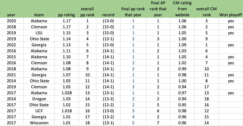
The #1 team of the era? 2020 Alabama. Here is the full list of every team in the playoff era that managed to get greater than a 1.0 playoffPredictor.com rating:

2020 Alabama was an incredible team that does not get their due because of COIVD. No close games at all – closest win was 15-points to Ole Miss. 8 blowouts, including both playoff games. Did not even play anyone ranked lower than #82.

2018 Clemson is on top of 2019 LSU because they played only 2 close games (Texas A&M and Syracuse), only 2 games with a normal victory margin (South Carolina and Boston College, 20-21 points each, which is right on the edge of blowout), and every other game was a >= 28-point blowout, including against #3 Notre Dame and #2 Alabama. I mean, who in the cfp era beats Alabama by 28 points? That list has one entry on it. I mean, there are only 2 other entries on the list that have beaten Bama by more than 7 points in the 9 years of the CFP era (2021 Georgia-15 points, and 2017 Auburn-12 points).

The only teams to make the list outside of the Alabama/Georgia/LSU/Clemson/Ohio State leadership are Oregon, UCF, and Wisconsin.

So back to 2019 LSU, why are they relatively low? Because before blowing out Oklahoma and beating Clemson in the playoff, they played 3 games all decided by 7 points or less (Texas, Auburn, Alabama). That lack of margin-of-victory hurts their overall resume. In fairness, this is a clear situation where Margin-of-Victory does not tell the correct story. In all three of those games LSU was in control and simply recovered an on-side kick by the opposition in order to turn a late 2-score game into a 1 score game and took knees to end those games. Maybe in another year I’ll switch the formula to time of victory and that will put 2019 LSU higher, but that is for another blog post. 2019 Ohio State was an incredible computer team that year, even with the single loss to Clemson. Better than 6 of the last 9 national champions. It would have been something special to see that 2019 Ohio State team take on 2019 LSU if that wide receiver had not stopped his route short.

Probabilities of a 7-game series

Ever wondered how odds map from a single game contest to a best of 7 series? For example, say you knew in any single game between team A and team B that team A will win 60% percent of the time. If they were to play a one game series on a neutral floor team A obviously advances 60% of the time. But what if they play a 7 games series (all on a neutral floor).  What do team A’s odds improve to?  

This can be computed analytically and straightforward. ChatGPT says to use the binomial distribution, but I’m not sure that’s 100% correct yet. Binomial will get you the probability team A gets exactly 5 wins in a 7 trials, but of course that can’t happen as after you win 4 the series is over. So, let’s just exhaust all possibilities between team H(favored) and team A(underdog):

For team H to win in 4 games there is one way: HHHH, total probability is p4  where p is defined as the probability team H wins any one game (60% from our original question).  0.64 = .1296 = 12.96% ≈13%.  Meaning there is a 13% team H will sweep. 

Team H can win in 5 games 4 different ways: HHHAH, HHAHH, HAHHH, AHHH.  Each has a probability of p4 (1-p) = 0.05184 in our scenario. Multiplying by the 4 ways to achieve that result leaves a total probability of 4p4 (1-p) = 20.736%.  

Team H can win in 6 games 10 different way and in 7 games 20 different ways (reader can check those for themselves), so final probability for team H to win a 7 game series is:

Where q is defined as (1-p)

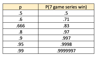
Run the numbers and you find that 60% for a single game translates into 71% for a seven-game series (71.0208% to be exact).  So, a 7 game series will draw out the better team by a benefit of 11% for a team that is already 10% better than a 50/50 coin flip.

Running the number for other values of p you get:

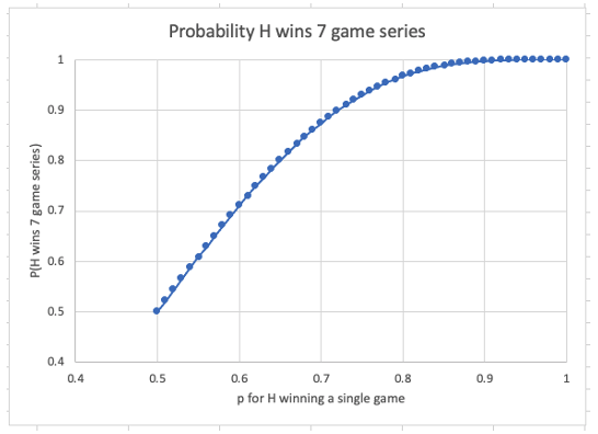
So it gives a 2x boost initially, with diminishing returns as you get past 80-90%. Charted out it looks like this:

To me its compelling at p=80% or so. p=80% becomes 97%. p=80% means the team is -400 – bet $400 to receive $500.   So—unless your team is a -400 favorite in game 1, don’t be too confident they will win the 7-game series.  In fact, you can extrapolate the series winning odds from the odds from game 1.  

Now, how about when team H wins the first 2 games?  I’ve heard it said then for team A to win becomes impossible because they have to win 4 of 5 games.  How likely is that? The formula there becomes:

For a p=.5 that works to 81%  Not very impossible at all, in fact will happen 1 our of 5 times.

Well, then why in the NBA when a team goes up 2-0 they win the series 95%? Because of course the team that goes up 2-0 is better than 50/50 against team B. More like p=0.66 – that gets you to 95% series wins after going up 2-0.     Note, p=0.66 gets you only to 81% for the series before the start of game 1.  

Summarizing the math:

If team A is 2x better (p(A)=.666, will win 2 times out of 3), then they win the series 81%.

If team A is 2x better (p(A)=.666, will win 2 times out of 3) and they win first 2, then they win the series 95%

If team A and team B are equal (50/50), then team A wins the series 50% (duh)

If team A and team B are equal (50/50) and team A wins the first 2, then team A wins the series 81%

If team A is worse (p(A)=.333) but wins first two games, they win the series 54%  — even though they are worse.

Bottom line – winning a 7-game series after going down 0-2 is not hard – as long as you are the better team!  Be twice as good and you have a 47% shot of pulling off the comeback.

Playoff probabilities via Monte-Carlo

I have added a product to the playoffPredictor.com site that visualizes the percentage chances a team has to make the college football playoff.

PlayoffPredictor.com was launched with the express belief that if you knew who was going to win future games, you could accurately predict the top 4 in the final poll. If you know (or can predict) that Alabama is going to beat Georgia in the SEC championship game, can you definitively predict if Georgia will still make the college football playoff? Yes, you can answer that if you know how all the other games pan out (like Baylor beating Oklahoma State for example, leaving that slot open for Georgia).

The next logical place to use that data would be to iterate through each future scheduled game and using the probabilities of each team to win, exhaustively calculating the probability of each team to win the college football playoff. Unfortunately exhaustive scenario modeling is virtual computational impossibility. If you tried to enumerate every possibility (just for wins and losses, not even for margin of victory) from week 8 till week 14, you have about ~450 games to model. Given that a game only has two possibilities for the winner, this works out to 2450 = 2.9*10135 scenarios to model. How big is 10 raised to the 135? Well, I have seen estimates of the number of atoms in the know universe anywhere from 1085 – 10110 , so 10135 is many orders of magnitude larger than the number of atoms in the universe, and would take trillions of years to compute.

So do we give up modeling future probabilities? No, we introduce Monte-Carlo simulations. The idea is that if we know percentage chances for an individual trial (say Ohio State beats Penn State 85% of the time), we simulate that trial and the other 449 games a large number of times, and calculate who actually made the top 4. This is much simpler because you only have to compute 450 * 1,000 = 450,000 = 4.5 * 105 computations, and that can be done in a matter of minutes.

So, the new product is on playoffPredictor.com. After week 6 I like how my calculated data matches with reasonable expectations. We have Ohio State and Clemson most likely to reach the cfp at ~65% (because the ease of their championship games), followed by Alabama and Georgia at ~50% and 40% respectively. Same boring top 4. The challengers around the ~25% mark are Mississippi, TCU, and USC, and then 13 teams under 20%, including Syracuse at 14%. Could Syracuse make it? Sure – imagine this scenario:

  • Tennessee beats Alabama twice (week 7 and SEC championship
  • Tennessee, Florida, and Mississippi State beat Georgia (weeks 9, 10 & 11)
  • Texas Tech and Baylor beat TCU (weeks 10 & 12)
  • UCLA and Oregon beat USC (week 12 and Pac12 championship)

You could end up with undefeated Syracuse, Ohio State, and Tennessee coupled with winners of the Big12 and Pac12 at 2-3 losses each, and a 2-loss Alabama. In that (unlikely) scenario, you put in Tennessee, Ohio State, Alabama, and Syracuse. And variations of that are exactly what the computer came up with 140 times out of the 1,000 simulated seasons.

Enjoy the new tool, compare it with ESPNs probabilities through the season, and drop me a line at @CiscoNeville if you have any thoughts on this new visualization.

Elo predictions for college football – base and divisor

Ever thought about chess ratings? The highest chess rating ever for a human is held by Magnus Carlsen at 2882. The lowest is shared by many people at 100. The United States Chess Federation initially aimed for an average club player to have a rating of 1500. There is no theoretical highest or lowest possible Elo rating (the best computers are at ~3500 and the negative ratings are theoretically possible, but those people will get kicked from tournaments, so they arbitrarily set 100 as a lowest possible rating).

This particular range of numbers from 100 – 3500 is a consequence of the base and divisor that Arpad Elo chose. The Elo rating system for chess uses a base of 10 and a divisor of 400. Why? According to wikipedia the 400 was chosen because Elo wanted a 200 rating point difference to mean that the stronger player would win about 75% of the time, and people assume that he used 10 as a base because we live in a base 10 world. Interestingly if he would have used base 9 then 200 points would exactly be a 75% chance of win, where base 10 is more like 76% :

1 /(1+9(200/400)) = .25

1 /(1+10(200/400)) ≈ .2402

But enough on Chess. I like the playoffPredictor mathematical formula that puts the teams between roughly 0 and 1 instead of 100 and 3500. But what base and divisor do I use with that system?

Last year I went with base equal to the week number (1-17) and a divisor of .4. The reason for the week number is because bases 2-3-4 don’t exponent out to crazy scenarios, so in week 2 when there is very little data it does not make such drastic judgements. The divisor I picked empirically, it seemed to fit the data and it was also a callout to Elo’s 400.

Really though I have been doing some fiddling and I think a base of 1000 and a divisor of 1 will work better. Here are some spreadsheet results.

Elo probabilities for different bases with constant divisor of 1

To read the above table, look at the row for 1000. This reads so if a team is better by .2 (like computer ratings of .9 and .7 for the 2 teams) then the .9 team as a 79.9% chance of winning. I need to model these against real life, but I feel this is a start.

Further for choosing a base and divisor the following are all equivalent pairs:

equivalent pairs for bases/divisors

So 1000 and 1 give the same result as 10000 and 1.3333, or 100 and .6666. In the same way 1000 and 3 give the same result as 100 and 2, or 10 and 1. Log math.

So I’m going to move to a base of 1000 and a divisor of 1. The divisor of 1 make sense — take that out of the equation. Then, what base should you use? Empirically 1000 seems to fit well. I need to backtest with data from week 13-14 when ratings are pretty established to see how the percentages mesh with Vegas. To do.

At a base of 1000 and divisor of 1, a team with a rating +.16 more than an opponent will have a 75% chance of winning. So in this sense +.16 corresponds to 200 points in chess Elo.

In my rating the teams will be normally distributed with a mean at 0.5 and a standard deviation around 0.25. Meaning teams that are separated by 1 standard deviation, the better team has a 85% chance at success. For example, the following teams are all about 1 sigma apart:

  • #1 Georgia (~1)
  • #20 BYU (~.75)
  • #70 Illinois (~.5)
  • #108 Tulane (~.25)
  • #129 1AA (FCS) (~0)

So Georgia has a 85% chance of beating BYU, BYU has a 85% chance of beating Illinois, Illinois has an 85% chance of beating Tulane, and Tulane has a 85% chance of beating a FCS school. Is that right? Not sure

Keeping with the logic, Georgia would have a 97% chance of beating Illinois [1/(1+1000^(-.5))]. BYU would have a 97% chance of beating Tulane. Are those right? I think so. Would need to check against Vegas.

tldr; PlayoffPredictor.com used to use week number and .4 for the base and divisor, but now uses 1000 for the base and 1 for the divisor.

Just how fast was Secretariat?

I’m a fan of Secretariat. I’m not sure why, but a lot of people are fascinated by this horse. I think that when you see greatness – something that is just clearly apart from all others, it just brings emotions out. Even Jack Nicklaus cried watching Secretariat win the Belmont in 1973, that should tell you something.

You can google quite a lot about how fast Secretariat was (37.7 mph / 2:24 flat for the Belmont), or even how big his heart was (22 pounds, when the average horse heart is about 9 pounds, and the next biggest horse heart on record is ~15 pounds), but those numbers, especially the speed numbers, are clinical. They don’t give the context to let you appreciate. Enter statistics:

It is a very easy statistical problem to look at all the Belmont winner times since 1925 (ever since the track was at its current 1.5 mile length). Secretariat is the record holder at 2 minutes and 24 seconds flat. The next closest horse is 2 minutes and 26 seconds flat. There are about 90 horses between 2:26 to 2:33. Here is the list:

 YEAR	HORSE	         time (seconds)	Z score	percentage
1973	Secretariat *	        144.00	-3.01	99.870%
1992	A.P. Indy	        146.00	-1.83	96.674%
1989	Easy Goer	        146.00	-1.83	96.674%
2001	Point Given	        146.40	-1.60	94.515%
1988	Risen Star	        146.40	-1.60	94.515%
1957	Gallant Man	        146.60	-1.48	93.080%
2015	American Pharoah *	146.70	-1.42	92.263%
1994	Tabasco Cat	        146.80	-1.36	91.373%
1978	Affirmed *	        146.80	-1.36	91.373%
1985	Creme Fraiche	        147.00	-1.25	89.370%
2021	Essential Quality	147.10	-1.19	88.250%
1990	Go And Go	        147.20	-1.13	87.049%
1984	Swale	                147.20	-1.13	87.049%
1968	Stage Door Johnny	147.20	-1.13	87.049%
2004	Birdstone	        147.40	-1.01	84.400%
2009	Summer Bird	        147.50	-0.95	82.950%
1999	Lemon Drop Kid	        147.80	-0.78	78.102%
1983	Caveat	               147.80	-0.78	78.102%
2006	Jazil	        	147.90	-0.72	76.325%
1991	Hansel	        	148.00	-0.66	74.472%
1972	Riva Ridge	       	148.00	-0.66	74.472%
2018	Justify *		148.20	-0.54	70.549%
2003	Empire Maker		148.20	-0.54	70.549%
1987	Bet Twice		148.20	-0.54	70.549%
1982	Conquistador Cielo	148.20	-0.54	70.549%
1948	Citation *		148.20	-0.54	70.549%
1943	Count Fleet *		148.20	-0.54	70.549%
1975	Avatar			148.20	-0.54	70.549%
2019	Sir Winston		148.30	-0.48	68.489%
1965	Hail To All		148.40	-0.42	66.370%
1964	Quadrangle		148.40	-0.42	66.370%
1959	Sword Dancer		148.40	-0.42	66.370%
2016	Creator	        	148.50	-0.36	64.197%
2014	Tonalist		148.50	-0.36	64.197%
2005	Afleet Alex		148.60	-0.30	61.977%
1979	Coastal	        	148.60	-0.30	61.977%
1953	Native Dancer		148.60	-0.30	61.977%
1950	Middleground		148.60	-0.30	61.977%
1937	War Admiral *		148.60	-0.30	61.977%
2007	Rags to Riches (f)	148.70	-0.25	59.717%
1997	Touch Gold		148.80	-0.19	57.424%
1996	Editor's Note		148.80	-0.19	57.424%
1969	Arts And Letters	148.80	-0.19	57.424%
1967	Damascus		148.80	-0.19	57.424%
1962	Jaipur	        	148.80	-0.19	57.424%
1998	Victory Gallop		149.00	-0.07	52.770%
1981	Summing	        	149.00	-0.07	52.770%
1976	Bold Forbes		149.00	-0.07	52.770%
1955	Nashua	        	149.00	-0.07	52.770%
1951	Counterpoint		149.00	-0.07	52.770%
1974	Little Current		149.20	0.05	48.078%
1961	Sherluck		149.20	0.05	48.078%
1942	Shut Out		149.20	0.05	48.078%
1934	Peace Chance		149.20	0.05	48.078%
1947	Phalanx	        	149.40	0.17	43.412%
1938	Pasteurized		149.40	0.17	43.412%
2002	Sarava	        	149.60	0.28	38.836%
1977	Seattle Slew *		149.60	0.28	38.836%
1966	Amberoid		149.60	0.28	38.836%
1960	Celtic Ash		149.60	0.28	38.836%
1940	Bimelech		149.60	0.28	38.836%
1939	Johnstown		149.60	0.28	38.836%
1931	Twenty Grand		149.60	0.28	38.836%
2008	Da' Tara		149.70	0.34	36.601%
1993	Colonial Affair		149.80	0.40	34.411%
1986	Danzig Connection	149.80	0.40	34.411%
1980	Temperence Hill		149.80	0.40	34.411%
1956	Needles	        	149.80	0.40	34.411%
2017	Tapwrit	        	150.00	0.52	30.189%
1936	Granville		150.00	0.52	30.189%
1963	Chateaugay		150.20	0.64	26.217%
1958	Cavan	        	150.20	0.64	26.217%
1952	One Count		150.20	0.64	26.217%
1949	Capot	        	150.20	0.64	26.217%
1945	Pavot	        	150.20	0.64	26.217%
2012	Union Rags		150.40	0.75	22.532%
1971	Pass Catcher		150.40	0.75	22.532%
1935	Omaha *	        	150.60	0.87	19.159%
2013	Palace Malice		150.70	0.93	17.595%
1954	High Gun		150.80	0.99	16.115%
1946	Assault *		150.80	0.99	16.115%
2011	Ruler On Ice		150.90	1.05	14.718%
2000	Commendable		151.00	1.11	13.405%
1941	Whirlaway *		151.00	1.11	13.405%
2010	Drosselmeyer		151.60	1.46	7.207%
1930	Gallant Fox *		151.60	1.46	7.207%
1995	Thunder Gulch		152.00	1.70	4.495%
1944	Bounding Home		152.20	1.81	3.487%
1926	Crusader		152.20	1.81	3.487%
1927	Chance Shot		152.40	1.93	2.672%
1933	Hurryoff		152.60	2.05	2.023%
1932	Faireno	        	152.80	2.17	1.513%
1929	Blue Larkspur		152.80	2.17	1.513%
1928	Vito	        	153.20	2.40	0.815%
1970	High Echelon		154.00		(mud)

Its trivial in Excel to compute a mean of this data set (149.12 seconds) and a standard deviation (sample) of 1.699 seconds. From there you can see a Z score of each winner. I left out 1970 as the track was filled with mud (you can see that race here) . Leaving 1970 out moves Secretariat from a -2.93 to a -3.01, a true -3 Z score event. How rare is that? basic statistics says 99.7% of all data is between -3<Z<+3. So there is .3%, spread .15% in each tail — or that Secretariat happens less than .15% of the time. 99.87% of all Belmont winners will be slower. Put that in perspective with days: 1/0.13% is 770 — or it will take, on average, 770 years for a horse to eclipse Secretariat

Now this data is not perfect, normally you need 200 data points to have a good sample (What Carter Worth taught me). However, it is quite good. I’m sure we can bring in the 2nd and 3rd place finishers to get ~300 data points and still have about the same mean and standard deviation, but I’ll leave that exercise for someone else. Note this data is normally distributed, period. The central limit theorem states that no matter how horserace speeds are distributed, when I pull samples those are normally distributed.

For comparison here is how the top 45 finishers fare – note the 2:26 horses are a 1 in 30 year event. We will see 3 of those in our lifetime. But unless you are sticking around for the year 2750, you are not going to see Secretariat’s record taken down.

Losing my pinball machine

My parents moved us in 1981 from Pittsburgh, PA to Birmingham, AL. I was not pleased at the time to move again and lose my friends, so my parents bought me this pinball machine, that I played with for 40 years.

space odyssey pinball

It was finally time to let it go, I sold it in an estate sale for my parents last month. The player 1 did not keep accurate score as the 1,000 wheel was broken, but the player 2 side did keep accurate score. Here is my last time flipping those flippers — 129,070. A very good score! At 150,000 it lit the special for the free extra play. In general any time I played and got over 100,000 I was happy

I loved this pinball machine, but time to let go. Paid $400 for it, sold for $1,250 (I netted 70% of that via the estate sale)

2021 holiday letter

Dear Friends & Family, Christmas 2021

2021 has been a year I’ll remember for the Aga family. Life is good, and we continue to watch with wonder as our kids grow into the young people God has in store for each one of them. But 2021 was also a year of a missed opportunity for me.

Austin (23) is turning into a world explorer. He spent May in Italy with the OU in Arezzo program, and subsequently graduated from OU in June with his degree in advertising. He took advantage of the work-from-home trend and decided to start his career by moving to Seattle, Washington where he teleworks for Global Gear, an OKC based apparel company. On weekends he is exploring Seattle and the Pacific Northwest and hopes to continue his career with a northwest agency in 2022.

Evan (20) is in his second year at OU, which feels like a first year since last year as a university freshman all his classes were virtual with closed buildings. This year the OU campus feels open again, and Evan is living in an apartment east of campus, with a pair of roommates he has known since kindergarten. He bikes to his classes for engineering a couple times each day, which is giving him great exercise. He has grown well over 6 feet tall, and is easily the tallest Aga. He likes to take quick sprints (he does a half-mile in under 3 minutes ), and he spends weekends with the OU academic bowl team, including tournaments in Oklahoma and Texas.

Addison (14) is in her 10th year of dance at Massay’s, and her 2nd year of cheer at Whittier Middle School.

Emerson (14) is playing point guard for the WMS 8th grade varsity basketball team. She has a great team and group of friends, and she practices and gets better each day.

Addison and Emerson came with Shelli and I to Portugal this summer, where we got to explore Lisbon and Porto. We rented a car for a week and made it to the mountains that separate Portugal from Spain.

Neville’s parents Hoshi and Nergish decided to move from Birmingham to Norman to be closer to their grandkids. They have settled into a senior living center in Norman and Neville gets to drop by throughout the week. It is a very different dynamic than having them 700 miles away. They have gotten to see one of Emerson’s basketball games and weekly lunches with their kids and grandkids.

Shelli’s parents have had a challenging 2021 with Donnie getting a cancer diagnosis, but the great news is that reasonably early detection has given him a good prognosis, and he is feeling better now than he has felt at any time this year.

Shelli is active daily in her local yoga studio, fit and strong as ever. She is practicing headstands and keeping our family on track with all the events, activities, and homework of the girls.

As for me, after running what is likely my final half-marathon in October, I found out I have a broken heart (literally, not figuratively) and will need surgery in 2022 . I will finish up my night MBA program from OU this summer. Work at Cisco is humming along fine, I am in my 13th year of architecting networks at OU/OSU and school districts around the state. I did have an opportunity to move to the beach in Daphne, AL. Really a dream job for me at this career stage — Cisco security in commercial covering Alabama, Mississippi, and Louisiana. Looking back now I am very upset with myself for turning it down. I think about that bungled opportunity daily. I thought I was putting my girls needs ahead of my needs, but in reality I did not show the leadership and vision that the head of a family should show. At least now I know what was the biggest mistake of my life. One day soon I do want to get back to Alabama and the beach.

We hope this letter finds you well and thriving. Best wishes for a joyous holiday season and an exciting 2022.

Neville, Shelli, Addison, Emerson, Austin and Evan

Cisco Catalyst 9300 RFID identification

New Cisco switches come with a RFID tag. Need to do inventory? No need to move the switch all around looking for serial numbers, just use a scanner and read them in as you enter the room!

I bought a sub $100 scanner on Amazon (Thincol RFID reader) . It works as a keyboard — when it comes into contact with a RFID tag it energizes the tag and types out the info on the tag. This particular scanner works only with windows (or in my case a windows VM via virtualbox).

I was trying to RFID a switch with this serial:

FCW2141L002
The serial number from show ver

And when I used the RFID scanner, it outputted this info:

36142D8D4000B1E343AEC98B4633183064000000000000000000
what the RFID scanner outputs when applied to the switch

So, how in the world do you get to the serial from that hex gobbledygook? Read on!

There is this article on cisco.com on RFID tag identification. It seems to be the only article out there. It has some good info in it, mostly behind the theory, but lite on practicality. What is output from the scanner is only the Electronic Physical Code (EPC) at 208 bits. The tag ID and user memory portion are not read/output (at least I could not get anything there). Of those 208 bits:

  • Bits 1-8 are for the EPC header and say ’36’ in hex (0x36)
  • Bits 9-11 are for the filter and read ‘0’ in hex (0x0)
  • Bits 12-14 are for the partition and read ‘5’ in hex (0x5)
  • Bits 15-34 are for the GS1 company prefix (whatever that is) and read on my switch ‘0B635’ in hex (0x0B635). Note this is different than the example given on cisco.com which is 7 characters: 0746320
  • Bits 35-58 are for some item reference (again, whatever that is) and read ‘0002C7’ in hex (0x0002C7)
  • Finally bits 59-135 are where the serial number is

This is very non-intuitive (hey, it’s Cisco, not Meraki). Speficially if you look at the first 2 bytes that come back on the scanner (3614) – the 36 maps exactly to 36 for the EPC header, but the next byte (14) the “1” maps to all bits 9-11 for the filter (all zeros) and 1/3 of the bits 12-14 for the partition (specifically the first 1 in 101). The first half of the “4” maps to the rest of the filter 01 and the last half of the “4” maps to the first part of the GS1 company prefix (00). Confused? Yes you are.

Now the simple thing to do is put the string you get back from the RFID scanner in a HEX to binary converter like this one. Then on the resulting string back will be 206 bits long, like this

11011000010100001011011000110101000000000000001011000111100011010000111010111011001001100010110100011000110011000110000011000001100100000000000000000000000000000000000000000000000000000000000000000000000000

Why 206 bits and not 208? There are 0 leading zeros you have to put in for the ’36’ on the EPC header. So add in 2 leading zeros and you get:

0011011000010100001011011000110101000000000000001011000111100011010000111010111011001001100010110100011000110011000110000011000001100100000000000000000000000000000000000000000000000000000000000000000000000000

Now that you have 208 bits, you want to grab bits 59-135 (because you want 77 bits starting at position 59). Getting that out gives you:

1000110 1000011 1010111 0110010 0110001 0110100 0110001 1001100 0110000 0110000 0110010

(spaces added every 7 bits for readability)

Then you take those bits (with the spaces every 7 characters) and put them into a binary to ASCII converter: and you get: FCW2141L002.

Voila! FCW2141L002 from 36142D8D4000B1E343AEC98B4633183064000000000000000000